Introduction
LlamaIndex provides powerful data connectors, indexing, and retrieval capabilities, and also supports agent workflows. Depending on your requirements, you can combine it with LangChain or LangGraph to connect knowledge retrieval with agent orchestration.
In simple terms, LlamaIndex is commonly used to build knowledge bases for retrieval-augmented generation (RAG).
First, install the required dependencies:
pip install llama-index llama-index-readers-file python-dotenv
Since version 0.10, LlamaIndex has been modularized into the core package (llama-index-core) and separate integrations for models, vector databases, and readers, such as llama-index-embeddings-openai and llama-index-llms-openai. In production, you can also install only the integrations you need to reduce unnecessary dependencies.
For learning and rapid prototyping, the llama-index starter package includes the core module and the OpenAI LLM and embedding integrations. This article uses llama-index 0.14.25, which no longer bundles file readers. The installation command therefore explicitly includes llama-index-readers-file and python-dotenv, which we use later to load .env. Readers for particular file formats may require additional dependencies.
Common Reader Classes
1. Reading Local Files with SimpleDirectoryReader
SimpleDirectoryReader is one of the most convenient and commonly used loaders in LlamaIndex. Give it a local directory path, and it scans the directory and delegates parsing to the appropriate tools based on file extensions, such as .txt, .pdf, .docx, .csv, .md, .pptx, .jpg, and .mp4. The results are standardized Document objects.
The following three parameters are frequently used with SimpleDirectoryReader. Other parameters are available in its reference documentation:
from llama_index.core import SimpleDirectoryReader
reader = SimpleDirectoryReader(
    input_dir="./data", # Input directory
    # input_files=["./data/1.txt","./data/2.pdf"] # Load only the specified files
    recursive=True, # Recursively scan subdirectories; defaults to False
    exclude=["*.tmp", "temp/*"]  # Exclude temporary files or directories
)
Then call reader.load_data() to obtain a list of documents:
documents = reader.load_data()
For this test, I placed a single paper, A3PRVR.pdf, in the data directory:

Next, print the length of documents:

The output is 9, matching the nine pages of this AAAI2026 paper. The default PDFReader in this example returns one Document per page. This is not true of every PDF loading approach: this reader also supports return_full_document=True to return the entire document.
Now inspect the structure of documents[0]:
from pprint import pprint
pprint(documents[0].dict())
The output is shown below. I have shortened the text field because it is too long:
{'class_name': 'Document',
 'embedding': None,
 'end_char_idx': None,
 'excluded_embed_metadata_keys': ['file_name',
                                  'file_type',
                                  'file_size',
                                  'creation_date',
                                  'last_modified_date',
                                  'last_accessed_date'],
 'excluded_llm_metadata_keys': ['file_name',
                                'file_type',
                                'file_size',
                                'creation_date',
                                'last_modified_date',
                                'last_accessed_date'],
 'id_': 'ffabb7ce-eab0-4878-99b0-aa20a43cc7aa',
 'metadata': {'creation_date': '2026-09-22',
              'file_name': 'A3PRVR.pdf',
              'file_path': 'E:\\glader\\AgentLearning\\05-LlamaIndex\\data\\A3PRVR.pdf',
              'file_size': 1075393,
              'file_type': 'application/pdf',
              'last_modified_date': '2026-07-01',
              'page_label': '1'},
 'metadata_seperator': '\n',
 'metadata_template': '{key}: {value}',
 'relationships': {},
 'start_char_idx': None,
 'text': 'Action-and-object Aware Alignment for Partially Relevant Video '
         'Retrieval\n'
         '...',
 'text_template': '{metadata_str}\n\n{content}'}
The two main properties are metadata and text, which represent the document metadata and text content, respectively.
By default, SimpleDirectoryReader does not extract embedded images from PDFs. If you need this functionality, configure an appropriate parser through file_extractor, or use tools such as LlamaParse or PyMuPDF. Refer to the relevant documentation for details.
However, SimpleDirectoryReader can load image files directly and return a list of ImageDocument objects. For example, I prepared a portrait of Stalin:

Run the following code:
img_documents = SimpleDirectoryReader(input_files=["./data/sidalin.jpg"]).load_data()
pprint(img_documents[0].dict())
print("=" * 10)
print(type(img_documents[0]))
The result is:
{'class_name': 'ImageDocument',
 'embedding': None,
 'end_char_idx': None,
 'excluded_embed_metadata_keys': ['file_name',
                                  'file_type',
                                  'file_size',
                                  'creation_date',
                                  'last_modified_date',
                                  'last_accessed_date'],
 'excluded_llm_metadata_keys': ['file_name',
                                'file_type',
                                'file_size',
                                'creation_date',
                                'last_modified_date',
                                'last_accessed_date'],
 'id_': '2ddc1bfb-6d7d-4e07-a742-cb4d052a58d5',
 'image': None,
 'image_mimetype': None,
 'image_path': 'data\\sidalin.jpg',
 'image_url': None,
 'metadata': {'creation_date': '2026-09-22',
              'file_name': 'sidalin.jpg',
              'file_path': 'data\\sidalin.jpg',
              'file_size': 23769,
              'file_type': 'image/jpeg',
              'last_modified_date': '2026-09-22'},
 'metadata_seperator': '\n',
 'metadata_template': '{key}: {value}',
 'relationships': {},
 'start_char_idx': None,
 'text': '',
 'text_embedding': None,
 'text_template': '{metadata_str}\n\n{content}'}
==========
<class 'llama_index.core.schema.ImageDocument'>
Notice that the image document has an empty text property.
In general, SimpleDirectoryReader looks up file extensions in its default reader mapping and delegates parsing to the matching reader. The default behavior is summarized below:
| Extension | Reader | Format |
|---|---|---|
.csv | PandasCSVReader | Comma-separated tabular data |
.docx | DocxReader | Microsoft Word documents |
.epub | EpubReader | EPUB e-books |
.hwp | HWPReader | Hangul word processor documents |
.ipynb | IPYNBReader | Jupyter notebooks |
.jpeg / .jpg / .png / .gif / .webp | ImageReader | Image files |
.mbox | MboxReader | MBOX mail archives |
.md | Generic text loading | Read as plain text by default; use file_extractor to specify MarkdownReader |
.mp3 / .mp4 | VideoAudioReader | Audio and video |
.pdf | PDFReader | PDF documents |
.ppt / .pptm / .pptx | PptxReader | Microsoft PowerPoint presentations |
.xls / .xlsx | PandasExcelReader | Excel spreadsheets |
| Unrecognized extensions | Generic text loading | Read as text, with UTF-8 as the default encoding; this does not automatically instantiate FlatReader |
-
Dependencies are loaded lazily. The default specialized reader mapping depends on
llama-index-readers-file. If that package is missing and no parser is supplied throughfile_extractor, loading falls back to generic text handling, which cannot correctly parse binary formats such as PDF. -
Mappings can change between versions. Supported extensions and reader classes may differ across LlamaIndex releases. Check the source for your installed version. This table is based on 0.14.25.
-
Custom overrides. Use the
file_extractorparameter ofSimpleDirectoryReaderto override or extend the default mapping.
For details about each specialized reader, refer to the LlamaIndex documentation or the documentation for its integration package.
2. Reading Web Pages with SimpleWebPageReader and BeautifulSoupWebReader
Both readers load content from web pages. Install their integration separately:
pip install llama-index-readers-web
(1) SimpleWebPageReader
SimpleWebPageReader is a basic web reader. It fetches pages using requests, and the html_to_text parameter determines whether HTML is converted into readable text.
For example:
from llama_index.readers.web import SimpleWebPageReader
from pprint import pprint
# Do not pass URLs to the constructor
reader = SimpleWebPageReader(html_to_text=True)
# Pass URLs to load_data()
documents = reader.load_data(
    urls=["https://memo.myyrh.com","https://mblog.mslxl.com","https://blog.galyoo.top/post/newera/"]
)
pprint(documents[0].dict())
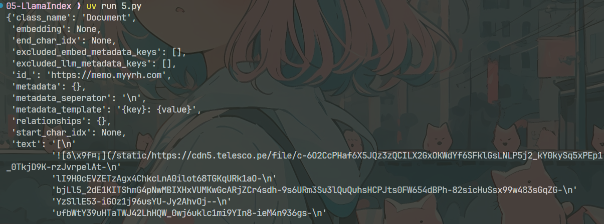
As shown above, the output is still difficult to read and contains garbled text.
(2) BeautifulSoupWebReader
from pprint import pprint
from llama_index.readers.web import BeautifulSoupWebReader
reader = BeautifulSoupWebReader()
documents = reader.load_data(urls=["https://memo.myyrh.com"
                 ,"https://mblog.mslxl.com",
                 "https://blog.galyoo.top/post/newera/"])
pprint(documents[0].dict())
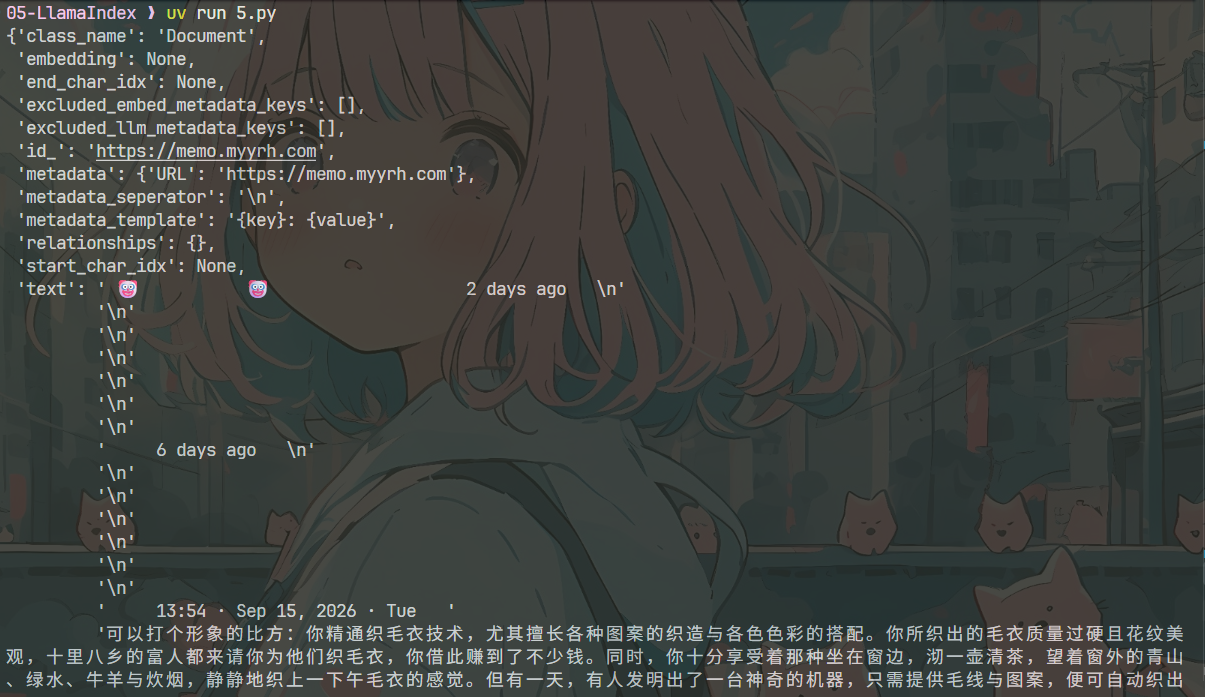
BeautifulSoupWebReader parses web pages with BeautifulSoup. For basic usage, pass urls. For sites without a specialized extraction rule, it extracts text from the entire page, which may include navigation and footers; it does not guarantee main-content-only extraction. For more precise extraction, customize site rules through website_extractor. Advanced usage and error handling are beyond the scope of this article.
3. Reading Databases with DatabaseReader
DatabaseReader reads database data and converts it into documents. It supports database systems such as MySQL, PostgreSQL, and SQLite.
For this MySQL example, first install:
pip install pymysql llama-index-readers-database
Here is a simple example using a database table prepared beforehand:
from llama_index.readers.database import DatabaseReader
reader = DatabaseReader(
    scheme="mysql+pymysql",
    host="localhost",
    port="3306",
    user="root",
    password="123456",
    dbname="test"
)
documents = reader.load_data(query="select * from user;")
print(documents)
The result is:

4. Writing a Custom Reader
When built-in or community readers do not meet your requirements, you can extend the system with a custom reader. Examples include calling an internal API, parsing an unusual proprietary format, or consuming data from a particular message queue.
LlamaIndex readers derive from the abstract BaseReader class. Writing a custom reader involves two main steps:
-
Inherit from
BaseReader. -
Override
load_data, implement your loading logic, and return a list ofDocumentobjects.
As a demonstration, we will write a reader for Markdown files, even though an existing reader is available:
from llama_index.core.readers.base import BaseReader
from llama_index.core import Document
# Custom reader for Markdown files
class MyMdReader(BaseReader):
    # Override load_data
    def load_data(self, file_path: str):
        with open(file_path, "r", encoding="utf-8") as f:
            text = f.read()
        return [Document(text=text[0:100]),Document(text=text[100:])]
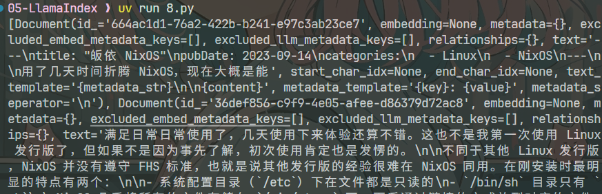
documents = MyMdReader().load_data("./data/index.md")
print(documents)
Text Splitting and Parsing
After loading, documents usually need further processing. Their granularity may be too coarse: a PDF page can contain body text, headers, footers, and references. Their length is also uncontrolled, so embedding or passing them directly to an LLM may exceed context limits or introduce retrieval noise. Before indexing, documents are therefore usually split into reasonably sized, semantically coherent Node objects. You can do this explicitly or let from_documents() handle it internally. LlamaIndex provides components such as TextSplitter and NodeParser for this purpose.
For the examples in this section, we use a NixOS introduction and its Markdown source.
Download index.md and place it in the data directory.
1. Splitting Text with TokenTextSplitter
Two common TokenTextSplitter parameters are chunk_size and chunk_overlap. chunk_size controls the maximum number of tokens in a chunk, while chunk_overlap specifies the overlap between neighboring chunks. Overlap helps retain context across boundaries, reducing the risk of losing important information when a sentence or passage is split. See the documentation for other parameters.
Test the following code:
from llama_index.core import SimpleDirectoryReader
from llama_index.core.node_parser import TokenTextSplitter
documents = SimpleDirectoryReader(input_files=["./data/index.md"]).load_data()
print(len(documents))
splitter = TokenTextSplitter(chunk_size=100, chunk_overlap=50)
nodes = splitter.get_nodes_from_documents(documents=documents)
print(len(nodes))
print("=" * 100)
print(nodes[10])
print("=" * 100)
print(nodes[11])
With chunk_size=100 and chunk_overlap=50, the output is:
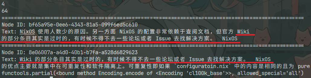
The red lines mark the overlapping content.
2. Splitting Text with SentenceSplitter
Using the same index.md, run:
from llama_index.core.node_parser import SentenceSplitter

splitter = SentenceSplitter(chunk_size=100, chunk_overlap=50)
nodes = splitter.get_nodes_from_documents(documents=documents)
print(len(nodes))
print("=" * 100)
print(nodes[10])
print("=" * 100)
print(nodes[11])
The result is:
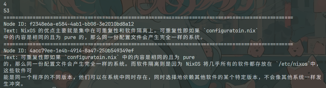
We use the same parameters as in the first example. The main difference is that SentenceSplitter prefers ending chunks at sentence boundaries rather than cutting a sentence in the middle.
Its main algorithm steps are illustrated below:
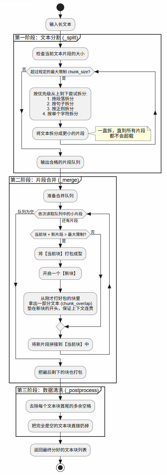
This keeps chunks within the chunk_size limit while preserving as much natural-language coherence as possible.
Beyond TokenTextSplitter and SentenceSplitter, LlamaIndex provides splitters for specific formats and more advanced scenarios. Here are a few examples; consult their documentation and test them against your own data:
- SemanticSplitterNodeParser: Uses embeddings to assess semantic similarity between neighboring sentences and places boundaries where topics change, rather than splitting solely by a fixed length.
- MarkdownNodeParser / HTMLNodeParser: Use document structure, such as Markdown headings or HTML tags, to split content while retaining structural context. These are also worth considering for
index.md. - SentenceWindowNodeParser: Creates sentence-level nodes and stores a window of surrounding sentences in metadata. After retrieval, use
MetadataReplacementPostProcessoror a similar step to supply the window as generation context, enabling small-chunk retrieval with larger-context generation. - CodeSplitter: Parses source code using an abstract syntax tree (AST), favoring function or class boundaries to avoid arbitrarily breaking code structure.
Building an Index and Generating Embeddings
We have loaded the data into documents and split them into nodes. Next, we convert the nodes into vectors and organize them into a structure for retrieval. In LlamaIndex, this step is called indexing.
The llama-index package installed earlier includes llama-index-embeddings-openai, so no additional installation is needed for this example.
First, define these environment variables:
OPENAI_API_KEY=your_api_key
OPENAI_API_BASE=your_api_base_url
VectorStoreIndex is the main class used here. Its common usage patterns are shown below.
1. Building an Index from Nodes
import httpx, json
from llama_index.embeddings.openai import OpenAIEmbedding
from llama_index.core import VectorStoreIndex
from llama_index.core.node_parser import SentenceSplitter
from llama_index.core import SimpleDirectoryReader
from dotenv import load_dotenv
load_dotenv()
documents = SimpleDirectoryReader(input_files=["./data/index.md"]).load_data()
splitter = SentenceSplitter(chunk_size=100, chunk_overlap=50)
nodes = splitter.get_nodes_from_documents(documents=documents)
# Inspect outgoing API requests
http_client = httpx.Client(
    event_hooks={
        "request": [
            lambda request: print(
                "\n===== Request =====\n",
                json.dumps(json.loads(request.read()), ensure_ascii=False, indent=2),
            )
        ],
        "response": [
            lambda response: print(
                "\n===== Response =====\n",
                json.dumps(json.loads(response.read()), ensure_ascii=False, indent=2),
            )
        ],
    }
)
embed_model = OpenAIEmbedding(
    model_name="qwen3.7-text-embedding", embed_batch_size=5, http_client=http_client
)
index = VectorStoreIndex(nodes=nodes, embed_model=embed_model)
We pass two main arguments to VectorStoreIndex: nodes, the chunks produced earlier, and embed_model, the embedding model instance that converts their content into vectors. This example uses qwen3.7-text-embedding with a batch size of 5, meaning each API request contains at most five nodes. The last batch may contain fewer. Model names and availability depend on your API provider.
The custom
http_clienthelps inspect API requests and responses while learning. You can omit it in normal application code.
The script prints several requests. Let us examine one batch:
===== Request =====
{
"input": [
"file_path: data\\index.md com/Misterio77/nix-starter-configs) 重构一下代码 配置文件在这: [mslxl/.dotfile](https://github.com/mslxl/.dotfile)  配置过程时,软件的主要从 [NixOS Package Search](https://nixos.org/nixos/packages.",
"file_path: data\\index.md dotfile)  配置过程时,软件的主要从 [NixOS Package Search](https://nixos.org/nixos/packages.html?channel=nixos-20.03) 中查询,部分与系统关系比较密切的通过 [Option](https://search.nixos.",
"file_path: data\\index.md org/nixos/packages.html?channel=nixos-20.03) 中查询,部分与系统关系比较密切的通过 [Option](https://search.nixos.org/options) 开启 使用中 NixOS 还是比较舒爽的,以安装 atuin 为例,如果是其他发行版安装可能还需要手动修改 `.",
"file_path: data\\index.md org/options) 开启 使用中 NixOS 还是比较舒爽的,以安装 atuin为例,如果是其他发行版安装可能还需要手动修改 `.zshrc` 文件,而 nix 只需要简单的添加 4 行配置,其他过程由 nix 自动完成。 ```nix programs.",
"file_path: data\\index.md zshrc` 文件,而 nix 只需要简单的添加 4 行配置,其他过程由 nix自动完成。 ```nix programs.atuin = { enable = true; enableBashIntegration = true; enableZshIntegration = true; };"
],
"model": "qwen3.7-text-embedding",
"encoding_format": "base64"
}
2026-10-03 11:53:51,482 - INFO - HTTP Request: POST https://ai.mygld.top/v1/embeddings "HTTP/1.1 200 OK"
===== Response =====
{
"object": "list",
"data": [
{
"object": "embedding",
"index": 0,
"embedding": "uf6YPG4yBj1BPH89gR......"
},
{
"object": "embedding",
"index": 1,
"embedding": "ghlMPJIw1jxFby......"
},
{
"object": "embedding",
"index": 2,
"embedding": "YoGTPJwupTxbNRE8k......"
},
{
"object": "embedding",
"index": 3,
"embedding": "t4JjPCWjnzzcH......"
},
{
"object": "embedding",
"index": 4,
"embedding": "yr2YPPuD9jwfjdU8......"
}
],
"model": "qwen3.7-text-embedding",
"usage": {
"prompt_tokens": 487,
"total_tokens": 487
},
"id": "ca28146a-0d05-923f-a667-a66608e059c4"
}
This request contains five chunks in the input array. Each combines file-path metadata with the chunk text. The "encoding_format": "base64" setting requests embeddings in base64 format.
The response contains five objects in data, each with a base64 embedding. Their values have been shortened for readability.
These strings are not base64-encoded versions of the original text. They are base64 representations of the vectors generated by the embedding model. The model transforms each chunk into a high-dimensional vector of floating-point numbers, for example:
[0.1234, -0.5271, 0.0812, …, 0.3145]
For transmission, these floating-point values can be represented as binary data and encoded as base64 strings. That is why the HTTP response contains values such as:
“uf6YPG4yBj1BPH89gR…”
The client decodes the base64 string into bytes, then reconstructs the floating-point vector for storage, similarity computation, and retrieval.
This representation can reduce transmission overhead compared with JSON floating-point arrays. High-dimensional embeddings contain many numbers, and JSON requires their textual representations plus separators and brackets. Base64 instead encodes the binary vector representation, avoiding decimal conversion of every value. It is therefore often useful when transmitting large numbers of high-dimensional embeddings.
The OpenAI Embeddings API also supports "encoding_format": "float" to return JSON floating-point arrays directly. Support for this option in third-party compatible APIs depends on their implementation.
To inspect the original vector behind a base64 value, I extracted the decoding logic from the OpenAI Python SDK called by LlamaIndex and adapted it into this script:
import array
import base64
import binascii
import json
def decode_embedding(encoded: str) -> list[float]:
    encoded = encoded.strip()
    if encoded.startswith('"'):
        encoded = json.loads(encoded)
    data = base64.b64decode(encoded, validate=True)
    if len(data) == 0 or len(data) % 4 != 0:
        raise ValueError(
            "Decoded data must contain a nonempty float32 vector (4 bytes per value)."
        )
    return array.array("f", data).tolist()

if __name__ == "__main__":
    try:
        vector = decode_embedding(input("Base64 embedding: "))
    except (ValueError, binascii.Error) as exc:
        print(f"Invalid embedding: {exc}")
        raise SystemExit(1)
    print(f"Dimensions: {len(vector)}")
    print("First 10 values: ") # Print the first 10 dimensions
    print(json.dumps(vector[:10], indent=2))
Run the script, paste one of the complete base64 values returned earlier, and inspect the output:
Dimensions: 1024
First 10 values:
[
  0.025365496054291725,
  0.03432830423116684,
  0.028960606083273888,
  -0.03395381569862366,
  -0.028785843402147293,
  -0.016377722844481468,
  0.044839005917310715,
  -0.09951463341712952,
  -0.011097405105829239,
  -0.007508536335080862
]
The resulting VectorStoreIndex object has the following structure:
index: VectorStoreIndex
├── index_struct: index mappings
│   └── vector ID → node ID
├── vector_store: vector storage
│   ├── node ID → embedding list
│   └── associated metadata
├── docstore: node storage
│   └── node ID → node object (text, metadata, etc.)
└── embed_model: model for embedding documents and queries
The resulting index supports the subsequent steps in our RAG workflow.
2. Building an Index Directly from Documents
Previously, we explicitly split Document objects into nodes and passed those nodes to VectorStoreIndex. This approach lets us inspect the chunks or filter and modify their metadata before generating embeddings.
If you do not need to handle nodes separately, use VectorStoreIndex.from_documents() to build an index directly from documents. The following example reuses the existing documents and embed_model:
from llama_index.core import VectorStoreIndex
from llama_index.core.node_parser import SentenceSplitter

index = VectorStoreIndex.from_documents(
    documents,
    embed_model=embed_model,
    transformations=[
        SentenceSplitter(chunk_size=100, chunk_overlap=50),
    ],
)
transformations specifies preprocessing steps. Here, we supply the same SentenceSplitter as before and let the framework perform splitting internally. If omitted, the global Settings.transformations configuration is used. With unmodified settings in the llama-index-core 0.14.25 version used here, the default is SentenceSplitter with chunk_size=1024 and chunk_overlap=200, both measured in tokens, not characters.
The default transformation pipeline is equivalent to:
transformations=[
    SentenceSplitter(chunk_size=1024, chunk_overlap=200),
]
Creating splitter = SentenceSplitter(chunk_size=100, chunk_overlap=50) separately does not change the global configuration. Omitting transformations therefore will not reuse that splitter. To use the earlier 100/50 settings, pass it explicitly as above or configure Settings.transformations. The default transformation pipeline handles splitting; the subsequent index-building step calls embed_model to generate vectors.
Building directly from documents does not skip splitting; it delegates splitting to the framework. Both approaches follow the same main pipeline:
Documents → Split into nodes → Generate embeddings → Build the index
| Construction method | Use case |
|---|---|
VectorStoreIndex(nodes=nodes, embed_model=embed_model) | Nodes already exist, or you need to inspect, filter, or modify them before embedding |
VectorStoreIndex.from_documents(documents, ...) | Start from documents and build the index using specified or default transformations |
These are the two main entry points to learn in this introductory tutorial. Choose one based on whether you need to process nodes separately; do not run both in sequence. Building both indexes from the same documents will usually make separate embedding requests rather than reuse vectors from the other index.
Other construction methods support additional use cases. Refer to the official documentation when your application needs them.
Persistent Storage
Without an external vector database, vectors, nodes, and index mappings are stored in memory by default. They are not automatically retained when the process exits. Reading, splitting, and embedding the documents on every startup takes time and causes repeated API charges. Instead, persist the built index locally and load it on subsequent runs.
1. Saving the Index Locally
Add this after building index:
index.set_index_id("nixos")
index.storage_context.persist(persist_dir="./storage")
First, assign an ID to the index. storage_context manages the document store, index store, vector stores, and related components. Calling persist() saves the default in-memory stores to the specified directory, rather than saving only an individual vector field.
./storage is relative to the working directory when the script runs. If you run it from 05-LlamaIndex, the files are saved in that directory’s storage folder.
With the default configuration, the resulting directory looks like this:
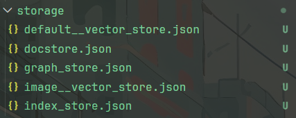
The following three files are most relevant to our text vector index:
| File | Contents |
|---|---|
docstore.json | Node text, metadata, and relationships |
index_store.json | Index IDs and types, and mappings from vector IDs to node IDs |
default__vector_store.json | Floating-point vectors and metadata used by the vector store |
image__vector_store.json and graph_store.json belong to other components in the default storage context. They may be empty in this text-only example; their presence does not mean image embeddings or a knowledge graph have been generated.
Persistence saves data that has already been built and does not call the embedding API again. Keep the entire storage directory for subsequent loading.
2. Loading the Index
Use a separate script to verify loading:
from llama_index.core import load_index_from_storage
from llama_index.core import StorageContext
from llama_index.embeddings.openai import OpenAIEmbedding
from dotenv import load_dotenv

load_dotenv()

embed_model = OpenAIEmbedding(model_name="qwen3.7-text-embedding", embed_batch_size=5)
storage_context = StorageContext.from_defaults(persist_dir="./storage")
index = load_index_from_storage(
    storage_context=storage_context, embed_model=embed_model, index_id="nixos"
)
print("Index ID:", index.index_id)
print("Loaded vector count:", len(index.vector_store.data.embedding_dict))
StorageContext.from_defaults() restores the storage components, and load_index_from_storage() reconstructs the index using its saved structure. Loading reuses the document vectors and does not make new embedding requests for those chunks.
The model object and API credentials are not restored from these files, so embed_model must still be configured. During retrieval, the user’s question needs to be embedded and compared with the stored document vectors.
Use the same embedding model and vector dimension settings for loading and querying as for building the index. Vectors from different models are not interchangeable, even when their dimensions match. If you change the model, regenerate the document vectors and save the index again.
The output confirms that loading succeeded:

Vector Retrieval
We have now loaded and split documents, generated embeddings, and saved and restored the index. Next, we find relevant chunks based on a user’s question. This step is called retrieval.
Retrieval returns relevant passages from the original documents, not answers generated by a chat model. Inspecting retrieval results separately helps verify that the knowledge base provides the necessary evidence before passing it to a chat model.
1. Creating a Retriever and Running a Query
Add the following after loading index in the previous section. The query and quoted source passages remain in Chinese because the example indexes a Chinese NixOS article:
retriever = index.as_retriever(similarity_top_k=3)
results = retriever.retrieve("为什么选择 NixOS?")

for i, result in enumerate(results, start=1):
    print(f"\n===== Retrieval result {i} =====")
    print("Node ID:", result.node.node_id)
    print("Similarity score:", result.score)
    print("Text:", result.node.text)
    print("Metadata:", result.node.metadata)
index.as_retriever() creates a retriever from the index. similarity_top_k=3 returns at most three candidate chunks, ordered by decreasing similarity. Creating the retriever alone does not send an embedding request; retrieve() embeds the query and performs retrieval.
The retrieval output is shown below:
===== Retrieval result 1 =====
Node ID: 531edc03-4647-4bca-8df2-ab2a08b05755
Similarity score: 0.7450133282241779
Text: NixOS 的优点主要就是集中在可重复性和软件隔离上。可重复性即如果 `configuratoin.nix` 中的内容是相同的且为 pure 的,那么同一份配置文件会产生完全一样的系统。
Metadata: {'file_path': 'data\\index.md', 'file_name': 'index.md', 'file_type': 'text/markdown', 'file_size': 8588, 'creation_date': '2026-09-23', 'last_modified_date': '2026-09-23'}

===== Retrieval result 2 =====
Node ID: 5405ace3-7e8b-4423-ba47-1e99a4189d79
Similarity score: 0.7446583632063953
Text: 因此 NixOS 也被称为滚不挂的系统(不作死的情况)。

实际上 NixOS 经常被人诟病占用硬盘,上手难度高,软件打包困难等。
Metadata: {'file_path': 'data\\index.md', 'file_name': 'index.md', 'file_type': 'text/markdown', 'file_size': 8588, 'creation_date': '2026-09-23', 'last_modified_date': '2026-09-23'}

===== Retrieval result 3 =====
Node ID: 8a1403f9-e272-4456-b633-16b1d8b5b570
Similarity score: 0.7301938186802789
Text: ---
title: "皈依 NixOS"
pubDate: 2023-09-14
categories:
  - Linux
  - NixOS
---

用了几天时间折腾 NixOS,现在大概是能满足日常日常使用了,几天使用下来体验还算不错。
Metadata: {'file_path': 'data\\index.md', 'file_name': 'index.md', 'file_type': 'text/markdown', 'file_size': 8588, 'creation_date': '2026-09-23', 'last_modified_date': '2026-09-23'}
The retrieval process can be summarized as follows:
User question
   ↓ Use the embedding model configured for the index
Query vector
   ↓ Compute similarity against stored document vectors
Select the highest-scoring vector records
   ↓ Retrieve nodes by ID
Return chunks, metadata, and similarity scores
2. Understanding NodeWithScore Results
results is a list of NodeWithScore objects. Each combines a retrieved node with its score:
results: list[NodeWithScore]
├── NodeWithScore
│   ├── node: retrieved node
│   │   ├── node_id: node ID
│   │   ├── text: chunk text
│   │   └── metadata: file path and other metadata
│   └── score: retrieval score
└── ...
Use result.node.text for the passage and result.score for its score. The node retains metadata from loading and splitting, which can later provide source files, page numbers, or other citation details. Available fields depend on the reader and document type.
3. Understanding similarity_top_k and Similarity Scores
similarity_top_k controls the number of candidates, not a minimum relevance requirement. A value of 3 means at most three results, without guaranteeing that all three answer the question. If fewer than three nodes are available, fewer may be returned.
With the default vector store and query mode used in this article, retrieval compares query and document vectors using cosine similarity and returns results in descending score order. Cosine similarity measures how closely two vector directions align. A higher score means greater proximity in this model’s embedding space.
A similarity score is not an answer accuracy rate or the probability that a passage is relevant. Even a high-scoring result must be inspected to determine whether it contains the required information. Other databases or retrieval modes may use different scoring methods, so the same interpretation or thresholds do not necessarily apply.
Keep the question fixed and compare similarity_top_k=1, 3, and 5. You only need to create a new retriever, not rebuild the document index:
query = "为什么选择 NixOS?"

for top_k in [1, 3, 5]:
    retriever = index.as_retriever(similarity_top_k=top_k)
    results = retriever.retrieve(query)

    print(f"\n===== top_k={top_k}, {len(results)} results returned =====")
    for result in results:
        print("Node ID:", result.node.node_id)
        print("Score:", result.score)
        print("Text:", result.node.text)
This code performs three retrieval operations and usually embeds the query for each one. Use it to explore the parameter’s effect. In applications, choose a suitable candidate count for the document and question types. Too few results may omit necessary evidence, while too many can introduce irrelevant passages and increase generation context length.
Finally, distinguish similarity-based sorting from reranking. The basic retrieval in this section already orders candidates by vector similarity, but does not call a separate reranking model. Reranking evaluates query–candidate relevance after initial retrieval and changes the order. It is an advanced retrieval optimization and is not covered here.
We can now retrieve relevant passages from the restored knowledge base. Passing the question and these passages to a chat model is the next step toward a RAG workflow that generates answers.