Interpretation of Differentiable Auxiliary Learning for Sketch Re-Identification

This paper is an AAAI-2024 article, titled “Differentiable Auxiliary Learning for Sketch Re-Identification.”

The paper proposes a network architecture called DALNet. This method generates a “sketch-like” intermediate auxiliary modality by performing background removal and edge detection enhancement on real photos, thereby bridging and aligning the sketch and photo modalities. Since the module responsible for generating this auxiliary modality is trainable and differentiable, supporting end-to-end optimization, the method is named “Differentiable Auxiliary Learning” (DAL).

1. Motivation

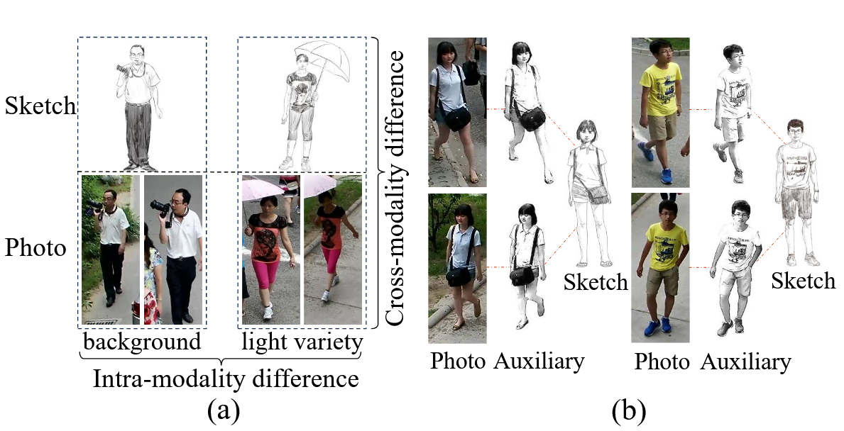
As shown in the figure above, the paper’s motivation is very clear and can be divided into two main points:

• The inter-modal differences between sketches and pedestrian images are too large. Can an intermediate modality be constructed to help bridge the gap between these two modalities?
• The intra-modal differences within sketches and pedestrian images are also significant. First, sketches of the same pedestrian may be drawn by different artists with diverse styles and varying levels of abstraction; additionally, photos of the same pedestrian under different cameras are severely affected by background clutter, illumination changes, and viewpoint/pose variations. This causes even photos of the same person to be far apart in the feature space, increasing matching difficulty.

To address the first problem, the paper constructs a “sketch-like” intermediate auxiliary modality as a bridge. This modality is generated through background removal and edge detection enhancement on real photos, effectively assisting in establishing inter-modal feature alignment. During the feature learning stage, the paper incorporates multi-modal collaborative constraints: using cross-modal circle loss to align the overall relationship among sketches, photos, and sketch-like images.

To address the second problem, the paper introduces intra-modal circle loss to specifically compress the distribution of the same identity within the same modality and increase the distance between different identities. For sketches, this reduces the impact caused by different artist styles; for real images, this reduces feature drift issues caused by illumination, background, and viewpoint/pose changes.

2. Method

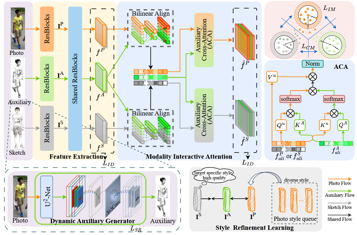
The overall framework of the model is shown in the figure above. In general, during the training phase, the Dynamic Auxiliary Generator (DAG) module first generates a sketch-like auxiliary modality image (this module is trainable and optimized through the $L_{SR}$ loss to make the generated auxiliary images adaptively approximate the target sketch style). Then, images from three modalities—sketches, auxiliary images, and real images—are encoded to extract features. The auxiliary modality features are then fused into the other two modalities, and through cross-attention mechanisms, shared semantic information between sketches and real images is strengthened to achieve fine-grained interactive fusion. Finally, classification loss and cross-modal/intra-modal circle loss jointly constrain the feature relationships and distributions of the three modalities. Below, I will analyze the details of each component.

Dynamic Auxiliary Generator (DAG)

This is the dynamic auxiliary generator module, whose function is to input a real image and output a sketch-like auxiliary image. Its principle is specifically shown in the following figure:

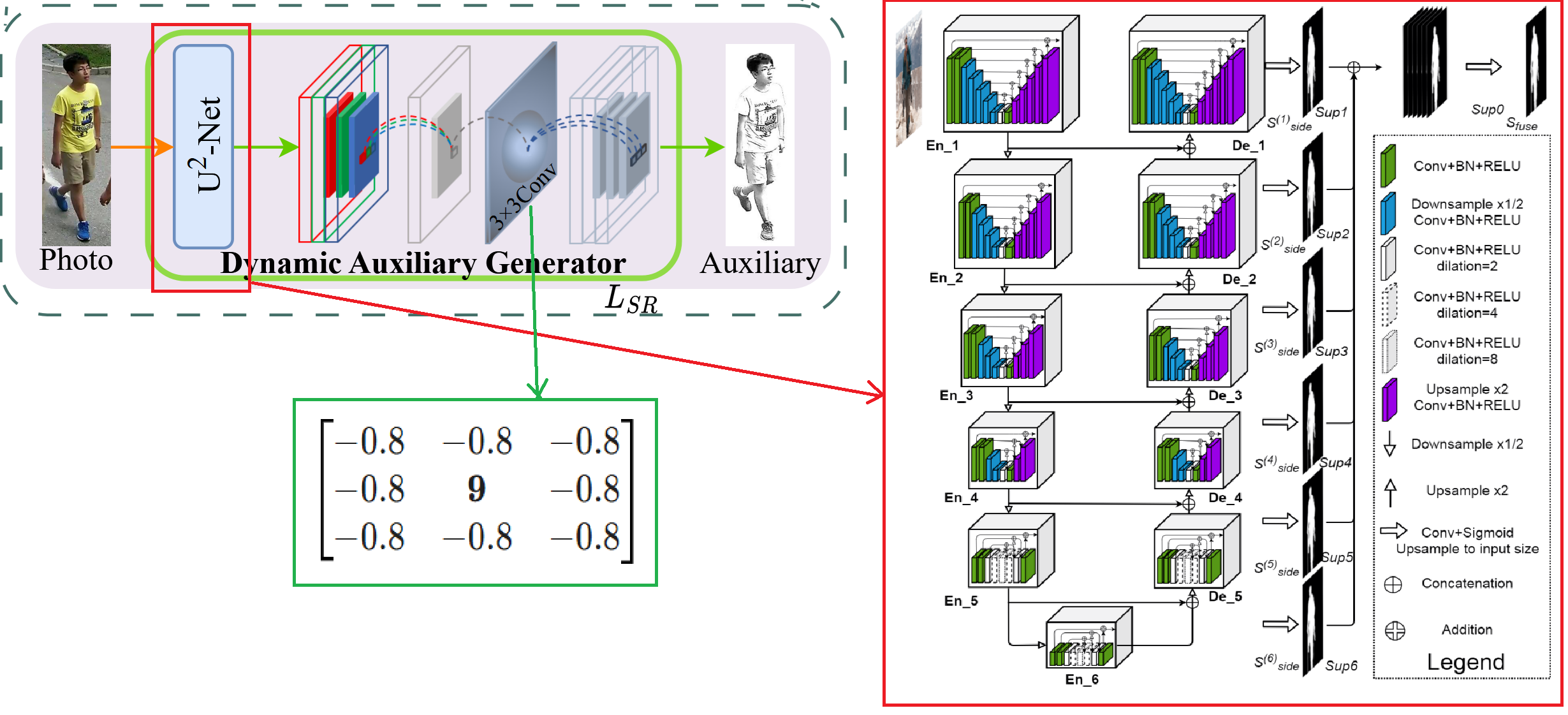
First, the real pedestrian image is input into the pre-trained U²-Net (whose network parameters remain frozen) to obtain a foreground segmentation mask matrix; then, this mask is used to filter the original image pixel by pixel, thereby retaining the pedestrian body and removing the background, obtaining a pedestrian image with the background removed. The specific structure of U²-Net is shown on the right side of the figure above. The reason it’s called U²-Net is that it is overall a U-Net-style encoder-decoder structure, but each encoding and decoding stage internally embeds a smaller U-Net (i.e., the RSU module, Residual U-block), equivalent to “U within U,” forming a cascade of two-layer U-shaped structures, hence named with U squared.

U²-Net generates multiple masks (side maps) from different scale side output layers during the decoding process. These masks correspond to foreground predictions at different resolutions: shallow side outputs focus more on edges and details, while high-level side outputs focus more on overall structure and semantic regions. During training, deep supervision is typically applied to these side outputs to stabilize convergence and enhance multi-scale segmentation capabilities. Finally, the multi-scale side outputs are fused (such as concatenation followed by convolution or weighted fusion) to obtain a final high-quality foreground mask for subsequent background removal.

After obtaining the pedestrian image with the background removed, it is still an RGB color image. Therefore, it first needs to be converted into a single-channel grayscale image through a 1×1 convolutional block, then passed through a 3×3 convolutional kernel for edge detection to enhance contour lines, making the grayscale image more approximate to a sketch, thereby generating a sketch-like auxiliary modality image. Here, this 3×3 convolutional kernel is trainable, which is also the only trainable and optimizable part of the DAG module, constrained by the loss function $L_{SR}$. The definition of this loss function will be analyzed in detail in the feature extraction module below. The convolutional kernel is initialized with a center value of 9 and surrounding 8 values of -0.8, first providing a stable “edge enhancement” prior, then adaptively adjusting the convolutional kernel weights during training according to downstream retrieval objectives, making the generated Auxiliary more conform to the contour expression of the sketch domain.

Feature Extraction

Next is the feature extraction module. As shown in the figure below, a three-stream ResNet-50 is used as the backbone to encode features for Photo, Auxiliary, and Sketch modalities respectively: each modality first passes through its own front-end ResBlocks (using the first two stages of ResNet-50) to extract low-level local features, obtaining global representations for the three streams; then the three-stream features are sent to the same set of “weight-shared” subsequent ResBlocks (using the remaining stages of ResNet-50) to learn higher-level, more semantically-oriented shared representations, preparing for subsequent modality interaction alignment.

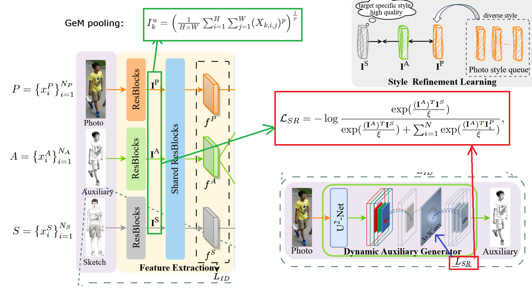
Specifically, define $P=\{x_i^P\}_{i=1}^{N_p}$ as the sample set of real images, where $N_p$ represents the number of samples. The $A$ and $S$ sets are similar, representing the sketch-like set and sketch set respectively.

Now, Photo, Auxiliary, and Sketch are put into their respective front-end ResBlocks to obtain three encoded feature maps. GeM Pooling operation is performed on these feature maps to obtain three pooled feature vectors $I^P$, $I^A$, and $I^S$ respectively. The specific formula is shown as $I_k^u$ in the figure above, where $u$ represents the modality, $k$ represents the current $k$-th channel, $H$ and $W$ represent the height and width of the feature map respectively, and $p$ is a learnable parameter. When $p$ is close to 1, the pooling will be more like “average pooling” (doing more uniform aggregation over the entire feature map); as $p$ gradually increases, the aggregation process will increasingly approach “max pooling” (emphasizing the positions with the strongest responses). The reason for using GeM Pooling is that it adaptively compromises between average pooling and max pooling with a learnable $p$: it can both preserve global structural information and highlight local discriminative regions more critical for pedestrian retrieval (such as clothing textures, contour details, etc.), thereby obtaining more robust and discriminative global representations in cross-modal matching.

After obtaining the three feature vectors, the paper calculates the style refinement loss function $L_{SR}$ (whose form is similar to InfoNCE), with the specific formula shown in the figure above. The purpose is to pull the Auxiliary generated by DAG from “photo style” toward “sketch style,” thereby optimizing the convolutional kernel parameters of the DAG module, without destroying the human body structure information it inherits from Photo. The specific approach is: using the style feature $I^A$ of the auxiliary modality as the anchor, treating the sketch style feature $I^S$ of the same identity as the only positive sample; in the denominator, only $I^S$ and a set of photo style features $\{I_i^P\}_{i=1}^{N}$ are included for comparison, without adding other sketch features, because the goal here is not to learn the “separability between sketches” (which belongs to identity discrimination and retrieval loss to handle), but to explicitly distinguish $I^A$ from the Photo domain and make it approach the Sketch domain: if the denominator introduces a large number of “other sketches,” the optimization will become making $I^A$ simultaneously far from these sketches (including sketches with similar styles to the target sketch), which can easily weaken the traction force of “approaching the sketch domain” and even introduce unnecessary identity and style mixing. Therefore, the comparison set of this loss is deliberately designed as “one sketch positive sample + multiple photo negative samples,” maximizing the similarity between $I^A$ and $I^S$ through softmax normalization with temperature coefficient $\xi$, minimizing the similarity between $I^A$ and each $I_i^P$, thereby achieving the style transfer constraint of “de-photo stylization + alignment toward sketch style.” The experimental details indicate that the temperature coefficient $\xi$ is set to 0.07.

Afterward, the feature maps from the three streams are sent to the same set of “weight-shared” subsequent ResBlocks to learn higher-level, more semantically-oriented shared representations, specifically denoted as $f^P$, $f^A$, and $f^S$, preparing for subsequent modality interaction alignment. Note here that what is sent to the subsequent ResBlocks is the original feature maps generated by the three streams, not the pooled $I^u$.

Modality Interactive Attention (MIA)

Next is the modality interactive attention module, specifically shown in the figure below. This module consists of two sub-modules: the Bilinear Align module and the Auxiliary Cross-Attention module.

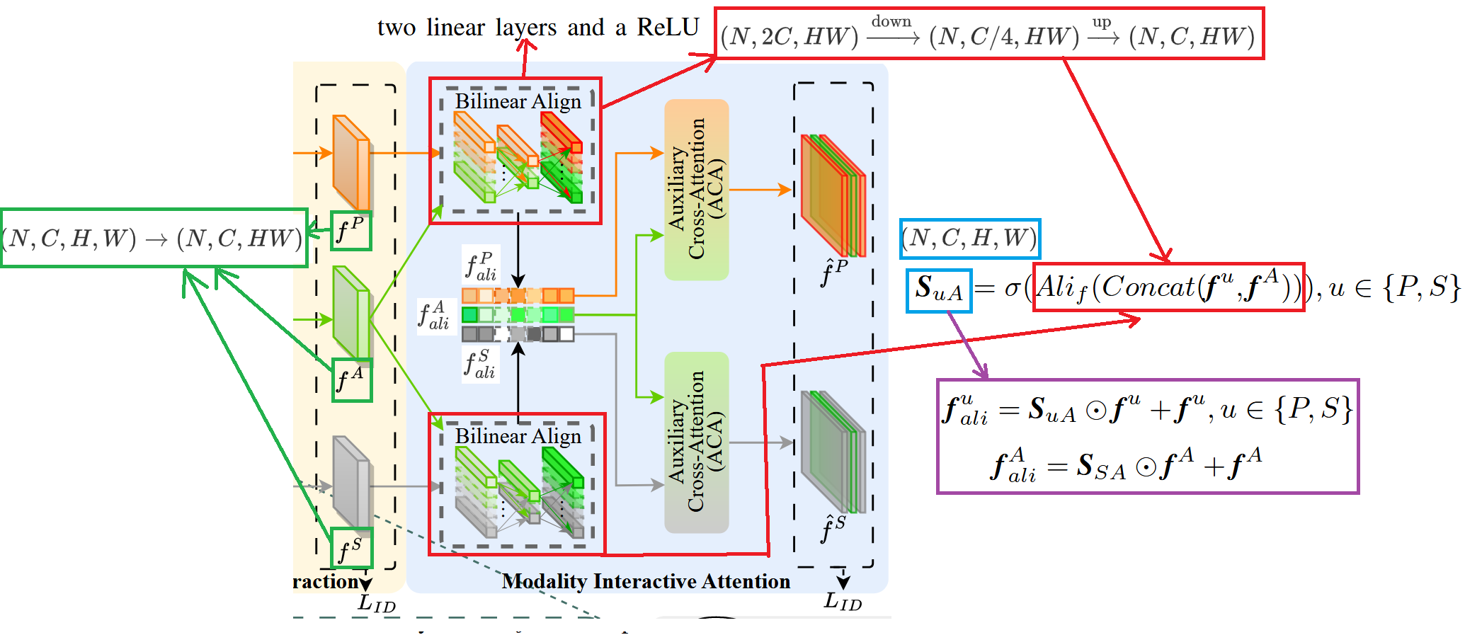
The Bilinear Align Module (BAM) is shown in the figure above. Its core function is to use the auxiliary modality feature map $f^A$ to calculate similarity weights $S_{uA}$ with the other two modality feature maps $f^P$ and $f^S$ (where $u\in\{P,S\}$). $S_{uA}$ can be understood as an “attention scoring map”: it characterizes the matching degree between the current modality features and auxiliary modality features at each spatial position and each channel. Positions with high matching will be assigned larger weights, thereby highlighting more reliable and consistent pedestrian structure cues when weighting features subsequently. Specifically, during calculation, $f^A$ and the target modality’s $f^u$ are first concatenated in the channel dimension, then sent to the bilinear alignment unit to model the second-order interaction relationship between the two, obtaining aligned responses. Then, through the sigmoid function $\sigma(\cdot)$, they are normalized to the $[0,1]$ range, forming similarity probability $S_{uA}$, which is used to perform attention weighting enhancement on $f^u$ and output aligned features.

The specific steps of bilinear alignment are shown in the figure above. First, tensor reshaping is required. The original $f^P$, $f^A$, and $f^S$ are actually tensors of shape $(N,C,H,W)$, where $N$ represents batch size, $C$ represents the number of channels, and $H$ and $W$ represent the height and width of the feature map respectively. First, the shape is adjusted to $(N,C,HW)$, then stacking and concatenation are performed to obtain a $(N,2C,HW)$ result concatenated on channels, as shown in the red box in the figure above. Taking the upper red box’s $f^P$ and $f^A$ as examples, after reshaping, these two feature maps are represented by a series of long strips, where the length extending into the screen can be abstracted as $HW$, and the number in the vertical direction can be represented as the number of channels $C$. When the two feature maps are stacked together, there are a total of $2C$ strips (C orange ones in the upper half, C green ones in the lower half). Then they enter a linear layer to compress the channels to $C/4$. The purpose is to first perform “dimensionality reduction compression” on the channel expression after two-modality concatenation as a lightweight bottleneck transformation without losing key information: because the number of channels becomes $2C$ after concatenation, if bilinear interaction is done directly in high-dimensional space, both parameter and computational costs will be large, and it’s easy to overfit. Therefore, the first linear layer first compresses the channels to $C/4$, which is equivalent to feature screening and information distillation, retaining the relevant components most helpful for two-modality alignment. Then it enters another linear layer to restore the channels back to $C$. The purpose is to remap the compressed “alignment relationship” back to the channel dimension consistent with the original backbone features, facilitating subsequent fusion/element-wise operations with original features, and ensuring that the output dimension matches subsequent modules (such as similarity estimation and attention weighting).

The calculated $S_{uA}$ will be reshaped back to $(N,C,H,W)$ shape to correspond one-to-one with the original feature map $f^u$ in spatial positions and channel dimensions. Subsequently, features are weighted and enhanced according to the alignment formula $f_{ali}^u = S_{uA}\odot f^u + f^u$: where $S_{uA}$ serves as attention weights, assigning higher responses to regions more consistent with the auxiliary modality and suppressing inconsistent or noisy regions, while preserving original information through the residual term. The finally obtained $f_{ali}^P$ and $f_{ali}^S$ are the Photo and Sketch feature maps guided and aligned by Auxiliary, providing “cleaner” and more alignable representations for subsequent ACA cross-attention interaction.

Meanwhile, to enable the auxiliary modality to also participate in bidirectional matching with “aligned, cleaner representations” during subsequent ACA cross-attention interaction (for example, using $f_{ali}^A$ as Key/Query to interact with $f_{ali}^P$ or $f_{ali}^S$), the paper also performs the same weighted residual enhancement on the auxiliary modality itself to obtain aligned auxiliary features $f_{ali}^A$. Specifically defined as using the similarity weight $S_{SA}$ between sketch and auxiliary modality to weight $f^A$: $f_{ali}^A = S_{SA}\odot f^A + f^A$.

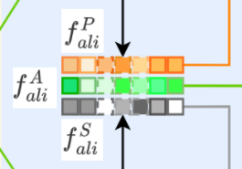
The final result is like this, where depth and shallowness represent the degree of attention to features. Deeper means stronger attention, while shallower means weaker. As for why some are dashed boxes, the paper doesn’t explain. I’ve consulted some drawing materials and learned that dashed lines may represent some common features under the three modalities.

Auxiliary Cross-Attention Module (ACA)

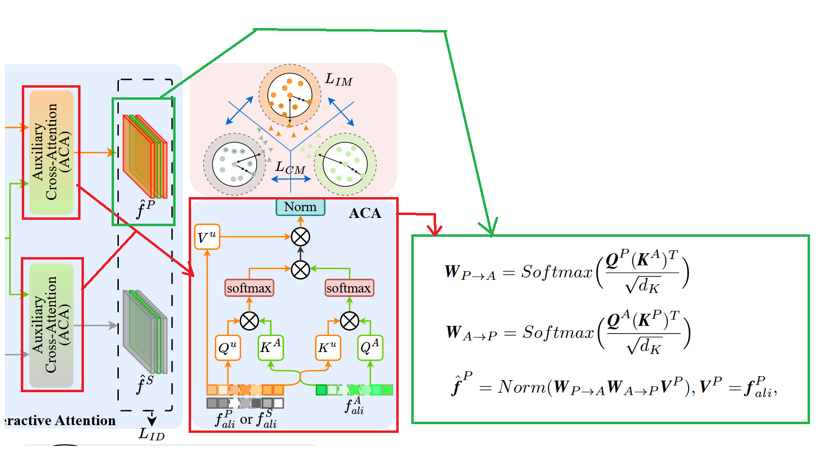
The purpose of ACA is not to “calculate another similarity score,” but to actually enable information exchange and fusion among the three modalities based on the aligned features obtained from BAM: the paper emphasizes that it “uses the auxiliary modality to guide the model in learning the distribution of modality-shared representations,” and can achieve significant information interaction and fusion between photo and sketch.

As shown in the figure above, taking “interaction between photo and auxiliary” as an example for specific calculation: the aligned features $f_{ali}^P$ and $f_{ali}^A$ output by BAM are respectively treated as Query and Key (denoted as $Q^P$ and $K^A$), then standard scaled dot-product attention is used to obtain matching weights from photo to auxiliary: $W_{P\rightarrow A} = \text{Softmax}\left(\frac{Q^P (K^A)^T}{\sqrt{d_K}}\right)$, where $d_K$ is the channel dimension of Key. At the same time, Query and Key are exchanged to obtain reverse matching weights: $W_{A\rightarrow P} = \text{Softmax}\left(\frac{Q^A (K^P)^T}{\sqrt{d_K}}\right)$.

With bidirectional weights, the paper uses a “round-trip consistency” method to refine photo features: using $V^P=f_{ali}^P$ as Value, multiplying $W_{P\rightarrow A}$ and $W_{A\rightarrow P}$ first, then weighting $V^P$, and finally performing LayerNorm to obtain photo features highlighted by the auxiliary modality: $\hat f^P = \text{Norm}\left(W_{P\rightarrow A} W_{A\rightarrow P} V^P\right),\quad V^P=f_{ali}^P.$ This can be understood as: first using $W_{P\rightarrow A}$ to find which positions or patterns in photo can find correspondence in auxiliary, then using $W_{A\rightarrow P}$ to “map this correspondence back” to confirm consistency, thereby more robustly strengthening the structural semantics shared by both and suppressing noise and inconsistent regions in each.

Similarly, performing the same bidirectional cross-attention on $f_{ali}^S$ and $f_{ali}^A$ yields the refined sketch features $\hat f^S$ guided by the auxiliary latent representation.

Multi-Modality Collaborative Learning

Multi-modality collaborative learning. This part mainly revolves around two types of losses: one is category loss, used to ensure that features of the three modalities have clear identity discriminability; the other is the circle loss series of metric learning losses, where cross-modal circle loss is used to constrain samples of different modalities but the same identity to approach each other in the feature space, and different identities to separate from each other, achieving overall inter-modal alignment; meanwhile, intra-modal circle loss is introduced to specifically compress the distribution of same-identity samples within the same modality and increase the distance between different identities, to alleviate intra-class dispersion problems caused by sketch style differences and photo viewpoint/illumination/background changes. The two work together to enable the model to simultaneously complete inter-modal and intra-modal alignment.

Category Loss

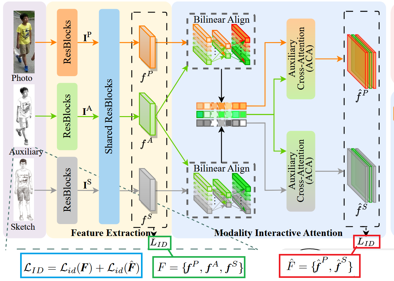
As shown in the figure above, the category (identity) loss uses $L_{ID}$. The purpose is to use “identity supervision” to pull the three modalities into the same separable identity space, allowing Photo/Auxiliary/Sketch of the same person to learn consistent identity patterns. The paper writes it as the sum of two parts: $L_{ID}=L_{id}(F)+L_{id}(\hat F)$, where $F=\{f^P,f^A,f^S\}$ represents the set of feature maps output by the three modalities through shared ResBlocks, $\hat F=\{\hat f^P,\hat f^S\}$ represents the set of Photo and Sketch feature maps enhanced through fine-grained interaction in MIA, and $L_{id}$ is the standard cross-entropy classification loss (using real identity labels for softmax classification supervision). The intuitive meaning of this design is: on one hand, directly constraining the three-modality basic representations extracted by the shared backbone to align at the identity level; on the other hand, also constraining the enhanced representations after auxiliary modality-guided interaction to still maintain correct identity discriminability, avoiding attention interaction “aligning” features to the wrong person or introducing identity-irrelevant deviations.

Circle Loss

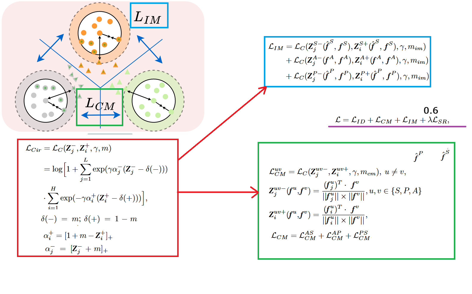
As shown in the figure above, the paper improves upon circle loss proposed in 2020, making it suitable for sketches and images, and designs two loss functions. One is $L_{CM}$, used for inter-modal alignment; the other is $L_{IM}$, used for intra-modal alignment.

The paper uses circle loss for metric learning constraints rather than the common triplet loss. The core reason is: Sketch Re-ID simultaneously has “huge cross-modal differences and extremely few samples per identity.” Simply using triplets often only provides local constraints on a small number of triplets, easily resulting in unstable optimization, strong dependence on hard samples, and the phenomenon of only considering cross-modal while ignoring intra-modal distribution. Circle loss, on the other hand, uses a unified form of “pairwise similarity optimization” to incorporate multiple pairs of positive and negative samples in a batch into optimization together, and emphasizes “harder” positive-negative pairs through adaptive weights $\alpha_i^+,\alpha_j^-$, making it more suitable for learning a more robust metric space with limited samples.

Let me first explain my understanding of the original circle loss. The original formula is shown in the red box in the figure above. It treats “similarity” as the optimization objective: for positive sample pairs formed by the same identity, similarity is denoted as $Z_i^+$ (hoping it to be as large as possible); for negative sample pairs formed by different identities, similarity is denoted as $Z_j^-$ (hoping it to be as small as possible). Therefore, its core is to simultaneously do two things: pull all $Z_i^+$ toward 1 (pull together same classes), while pulling all $Z_j^-$ toward 0 or even smaller (push apart different classes). It puts positive pairs and negative pairs into exponential functions separately for weighted summation: the exponential part of the positive pair term is roughly $-\gamma \alpha_i^+(Z_i^+ - \delta(+))$. When the similarity $Z_i^+$ of a certain positive pair is not large enough and is lower than the expected threshold $\delta(+)$, the bracket is negative, the exponential term becomes larger, contributing more to the loss, thus backpropagation will strongly push this positive pair to become more similar. Conversely, if $Z_i^+$ is already very large, exceeding $\delta(+)$, the contribution of this term becomes smaller, indicating that “easy positive samples” will not be over-optimized. The exponential part of the negative pair term is $\gamma \alpha_j^-(Z_j^- - \delta(-))$. When the similarity $Z_j^-$ of a certain negative pair is high, exceeding the threshold $\delta(-)$, this term will rapidly increase, and the loss will pay more attention to these “hard negative samples,” thereby pushing their similarity down. If the negative pair is already very small (already separated), its contribution will be automatically suppressed. Here, $\delta(+)=1-m$ and $\delta(-)=m$ are controlled by margin $m$, which is equivalent to setting a “passing line” for positive and negative pairs respectively, requiring positive pair similarity to exceed $1-m$ as much as possible, and negative pair similarity to be below $m$ as much as possible. $\gamma$ is the scale coefficient, used to control the “strength/steepness” of optimization. The most critical adaptive weights are $\alpha_i^+=[1+m-Z_i^+]_+$ and $\alpha_j^-=[Z_j^-+m]_+$: they will make positive pairs with unsatisfactory similarity ($Z_i^+$ small) and negative pairs most easily confused ($Z_j^-$ large) obtain larger weights, thereby naturally shifting the training focus to “hard sample pairs.” This is why circle loss can simultaneously achieve “pulling together same classes, pushing apart different classes” and be more stable.

Based on this, the paper further extends the “pairwise similarity optimization” idea of circle loss to the three-modality scenario and designs corresponding solutions for the two core contradictions of sketch Re-ID. First is inter-modal alignment $L_{CM}$: it no longer only constructs positive-negative pairs within the same modality, but directly calculates similarity between different modalities to construct positive-negative pairs, that is, changing $Z_i^+$ and $Z_j^-$ to cross-modal cosine similarities $Z_i^{uv+}(f^u,f^v)$ and $Z_j^{uv-}(f^u,f^v)$ ($u\neq v,;u,v\in\{S,P,A\}$), and applying circle loss constraints to the three groups of modality pairs $AS$, $AP$, $PS$ and then summing them. The intuitive purpose of doing this is: sketch, photo, and auxiliary of the same identity should be close to each other in the feature space, while different identities should be separated. Moreover, because auxiliary is in the “sketch-like” intermediate state, it simultaneously participates in the alignment of $AS$ and $AP$, playing a bridging role during optimization, indirectly reducing the alignment difficulty of $PS$. The specific formula is shown in the green box in the figure above.

However, if only $L_{CM}$ is used, the model often focuses its optimization on “cross-modal differences,” resulting in the distribution of the same identity within each modality still possibly being very scattered (for example, photos of the same person from different cameras are still far apart, or sketches by different artists still have large style differences), thereby learning a suboptimal latent space. Therefore, the paper adds intra-modal alignment $L_{IM}$: it still uses the form of circle loss, but constructs positive-negative pairs by constraining within the same modality. To create more powerful supervision with few samples, it pairs features before interaction $f^u$ with features after interaction $\hat f^u$ within the same modality to construct positive sample pairs (the same identity should be consistent), while selecting the most easily confused different-identity pairs as negative sample pairs. In this way, $L_{CM}$ is responsible for pulling different modalities into the same metric space to complete inter-modal alignment, while $L_{IM}$ is responsible for compressing intra-class dispersion and increasing inter-class gaps within each modality. The two work together to simultaneously alleviate both “cross-modal gap” and “large intra-modal differences.” The specific formula is shown in the blue box in the figure above.

In the experimental details, the parameter settings are $m_{cm}=0.25$, $m_{im}=0.5$, $\gamma=64$.

The total loss function is the sum of the above four loss functions, namely $L=L_{ID}+L_{CM}+L_{IM}+λL_{SR}$, where $λ = 0.6$.

3. Experiments

Dataset Configuration

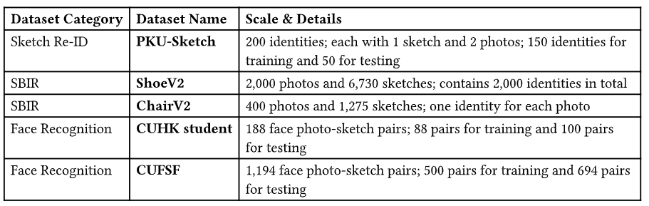
As shown in the figure above, the paper uses the above 5 datasets.

Ablation Experiments

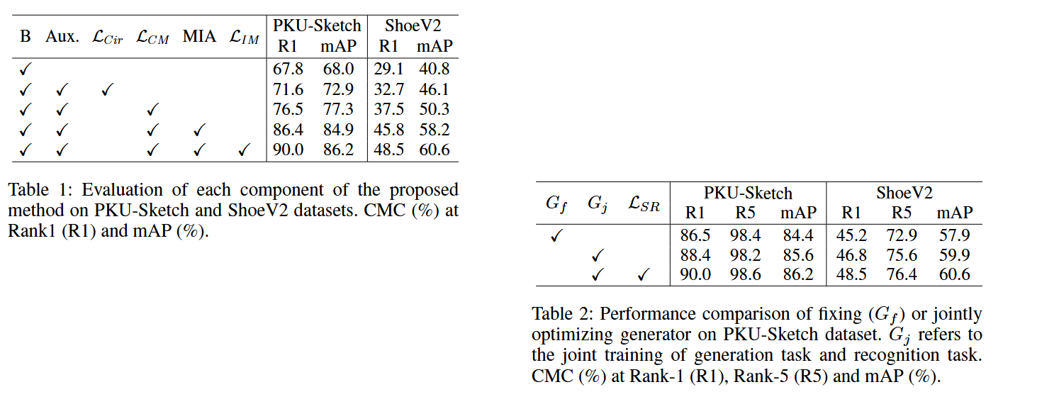
Table 1 above shows ablation experiments conducted on the PKU-Sketch and ShoeV2 datasets, where B represents Baseline. The paper explains that the Baseline here is “ResNet-50 trained with only identity loss.” Aux. indicates whether the auxiliary modality is introduced. $L_{Cir}$ represents the original circle loss, followed by the loss functions and modules designed by the paper. It can be seen that when using the complete model and loss functions proposed by the paper, all indicators are highest.

Table 2 above is to verify the impact of whether the DAG module participates in joint training updates on the entire model. $G_f$ represents fixed parameters, and $G_j$ represents parameters participating in training optimization, which refers to the convolutional kernel parameters. $L_{SR}$ refers to the style refinement loss. It can be seen that when using the $L_{SR}$ loss function to optimize the parameters of the DAG module during training, the model achieves the best performance with the highest indicators.

Comparison Experiments

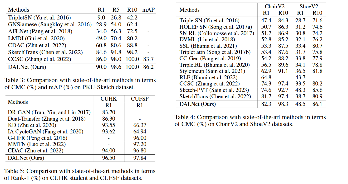
Tables 3-5 above compare with current SoTA models on different datasets. It can be seen that regardless of which dataset, the model proposed in this paper achieves the highest indicators.

Visualization Display

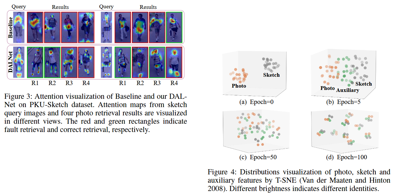
Figure 3 performs “attention visualization comparison.” The paper uses XGrad-CAM to draw attention heatmaps for two sketch queries from different viewpoints and their respective top-4 retrieved photo results, marking incorrect and correct retrievals with red and green boxes respectively. The conclusion is intuitive: the Baseline’s attention easily ignores truly relevant regions between sketches and photos, especially being interfered by some similar local features when scenes and poses change. DALNet, on the other hand, can simultaneously focus on more “cross-modally shared” human body cues (such as key facial regions, clothing textures, bags, badges, etc.), so there are more correct retrievals (green boxes).

Figure 4 performs “visualization of feature distribution alignment process.” The paper randomly selects 10 identities from PKU-Sketch and uses t-SNE to draw the feature distributions of the three modalities at different training epochs (brightness distinguishes different identities). The phenomenon is: at epoch=0, the distributions of photo (orange) and sketch (gray) are very different; as training progresses, auxiliary (green) acts like a “bridge” connecting the two; by epoch=50, photo and sketch gradually converge, with tighter intra-class and wider inter-class separations. Finally, at epoch=100, auxiliary features converge to their respective identity centers, indicating that the model has learned stronger identity discriminability and aligned the three-modality distributions.

Conclusion

This paper addresses the problems of large cross-modal gaps and severe intra-modal variations in sketch-based person re-identification by proposing DALNet: first, DAG generates a “sketch-like” auxiliary modality from real photos as a bridge; then a three-stream shared backbone extracts features, and through MIA, fine-grained cross-modal interactive fusion is achieved under the guidance of the auxiliary modality. Finally, classification loss and improved circle loss (including both cross-modal and intra-modal) are jointly optimized to achieve simultaneous inter-modal and intra-modal alignment.

The innovation lies in introducing trainable dynamic auxiliary modality generation and style refinement constraints to reduce modality differences, and designing the entire collaborative learning mechanism of “auxiliary-guided interactive attention and cross-modal and intra-modal circle loss,” making feature distribution alignment more stable and retrieval performance stronger.